kufreu.github.io
repository for geography work and other things completed by kufre u.
zonal statistics and land cover in chicago
Using a high-resolution land cover
raster
of Cook County obtained from the data hub of the Chicago Metropolitan
Agency for Planning (CMAP), I’m going to try to pass some time by seeing
how much tree canopy each tract in Chicago has with zonal statistics.
There are many ways to go about calculating zonal statistics, such as
using packages in R like exactexractr and stars, though here I have
have decided on using rasterstats and other packages in Python to do
so because it is rather straightforward. The first step was to import
the necessary libraries for this analysis.
import pandas as pd
import geopandas as gpd
import rasterio as rio
from matplotlib import pyplot as plt
from rasterstats import zonal_stats
The next and somewhat important step is to find data to spatially aggregate the land cover by. For this I have chosen to use census tracts boudaries in Chicago obtained from the City’s data portal. In the code chunk below, the census tracts are read and reprojected to the coordinate reference system of the land cover raster.
raster = 'cookcountylandcover2010\landcover_2010_cookcounty.img'

with rio.open(raster) as src:
    chicago = gpd.read_file('https://data.cityofchicago.org/api/geospatial/5jrd-6zik?method=export&format=GeoJSON').to_crs(src.crs)
zonal_stats from rasterstats can not only treat rasters as
categorical, which is important in this as my only concern is the pixel
count of each land cover class, but it has a parameter to map
categorical names to the pixel values with a dictionary. I can use the
attribute table from the raster to take advantage of this.
dbf = gpd.read_file('cookcountylandcover2010\landcover_2010_cookcounty.img.vat.dbf')

dbf
##    Value         Count                 Class geometry
## 0      0  5.926896e+09                  None     None
## 1      1  1.899942e+09           Tree Canopy     None
## 2      2  2.098441e+09           Grass/Shrub     None
## 3      3  1.586455e+08             Bare Soil     None
## 4      4  1.728156e+08                 Water     None
## 5      5  8.906310e+08             Buildings     None
## 6      6  6.564253e+08       Roads/Railroads     None
## 7      7  7.981709e+08  Other Paved Surfaces     None
I can see here how the values map to the different land cover classes. What will need to be done is to clean up the land cover classes for use as column names and to create a dictionary with the pixel values as keys and the classes as values.
classes = [str(x).lower().replace('/','_').replace(' ','_') for x in dbf['Class']]

land_cover = dict(zip(dbf['Value'].tolist(), classes))
Now that I have the dictionary with value-class pairs, I can use
zonal_stats.
zonal = zonal_stats(chicago,raster,categorical = True, nodata = 0, category_map = land_cover)

zonal[0]
## {'tree_canopy': 758410, 'grass_shrub': 1154562, 'bare_soil': 279572, 'buildings': 865204, 'roads_railroads': 1030389, 'other_paved_surfaces': 1209606}
For each census tract, a dictionary is created with a pixel count of the
land cover class found within the tract. Before doing this, however, I
needed to create a somewhat empty DataFrame which to put the values
from zonal_stats into. The categorical names from land_cover were
used as column names in this DataFrame and geoid10 was added to
identify each tract and to allow for joins, though the index of
DataFrame could also be used for the latter.
zeros = [0] * len(chicago)

results = pd.DataFrame(dict((v,zeros) for k,v in land_cover.items()))

results.insert(0,'geoid10', chicago['geoid10'])

results
##          geoid10  none  ...  roads_railroads  other_paved_surfaces
## 0    17031842400     0  ...                0                     0
## 1    17031840300     0  ...                0                     0
## 2    17031841100     0  ...                0                     0
## 3    17031841200     0  ...                0                     0
## 4    17031839000     0  ...                0                     0
## ..           ...   ...  ...              ...                   ...
## 796  17031070400     0  ...                0                     0
## 797  17031070500     0  ...                0                     0
## 798  17031130300     0  ...                0                     0
## 799  17031292200     0  ...                0                     0
## 800  17031630900     0  ...                0                     0
##
## [801 rows x 9 columns]
With the DataFrame created, what is next is to input the data using a
loop. There is most definitely a better way of doing this, both using
the results from zonal_stats or creating a DataFrame from a list of
dictionaries, though this way was still trouble-free. The values are
multiplied by four in the loop because the spatial resolution of the
raster is 2 survey feet.
for i in range(len(zonal)):
    row = zonal[i]
    for j in list(row.keys()):
        results.at[i,j] = row.get(j) * 4

results
##          geoid10  none  ...  roads_railroads  other_paved_surfaces
## 0    17031842400     0  ...          4121556               4838424
## 1    17031840300     0  ...          2115644               1821184
## 2    17031841100     0  ...          3599176               3002572
## 3    17031841200     0  ...          1717168               1635884
## 4    17031839000     0  ...           922564               1147704
## ..           ...   ...  ...              ...                   ...
## 796  17031070400     0  ...           485496                444696
## 797  17031070500     0  ...           385808                393256
## 798  17031130300     0  ...           868876                754644
## 799  17031292200     0  ...           730128                619612
## 800  17031630900     0  ...           907252               1704864
##
## [801 rows x 9 columns]
The results can now be joined to the tracts and the tree coverage of
each tract can be determined by dividing tree_canopy by the tract
area.
chicago = chicago.merge(results, how = 'left', on = 'geoid10')

chicago['pct_canopy'] = chicago['tree_canopy'] / chicago.area * 100
I can take a quick look at the tracts to see if pct_canopy appears to
be reasonable.
fig, ax = plt.subplots(1,1)
ax.axes.xaxis.set_visible(False)
ax.axes.yaxis.set_visible(False)

chicago.plot(column='pct_canopy',
             legend=True,
             ax = ax,
             legend_kwds={'label': "Canopy Cover"}
             )
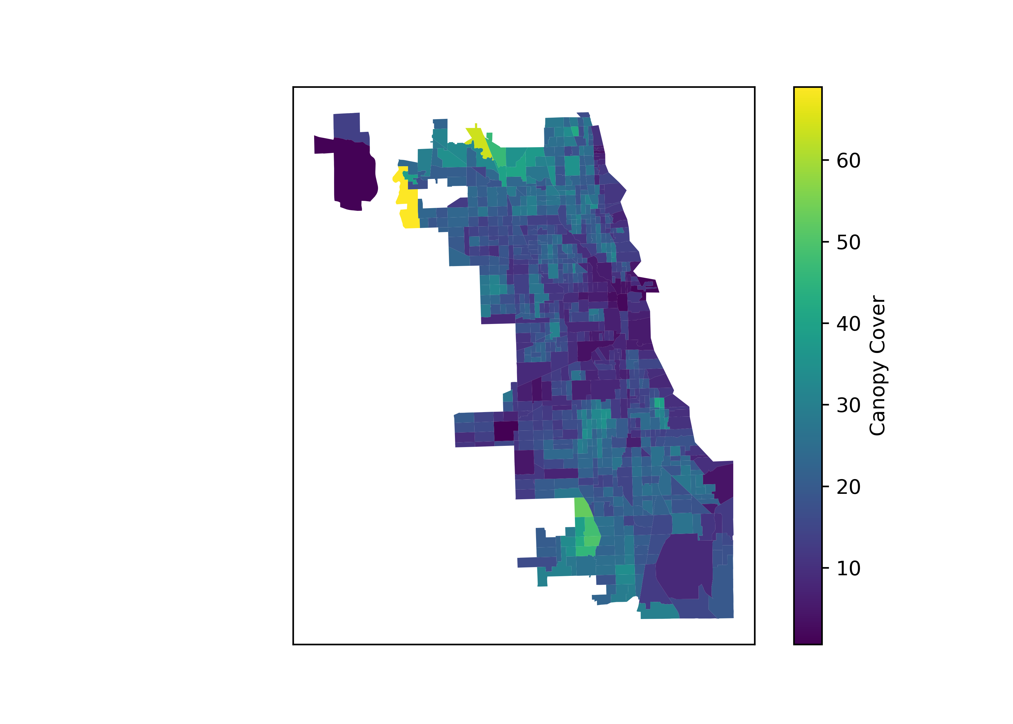
Although a pattern can be seen in the distribution of tree canopy in the
city, such as there being less tree coverage in and around the loop,
this map does not go as far as showing if and how this distribution maps
to race in Chicago. Possibly in the future I’ll continue this short
analysis in R by using tidycensus to collect demographic data for the
city. For now I will save the results.
results.to_csv('chicago_land_cover.csv')
chicago.to_file('chicago.gpkg', layer ='land_cover', driver="GPKG")